1    

2    

3    

4    

5    

6    

7    

Supervised Learning

The (fictional) information technology company JCN Corporation is reinventing itself and changing its focus to artificial intelligence and cloud computing. As part of managing its talent during this enterprise transformation, it is conducting a machine learning project to estimate the expertise of its employees from a variety of data sources such as self-assessments of skills, work artifacts (patents, publications, software documentation, service claims, sales opportunities, etc.), internal non-private social media posts, and tabular data records including the employee’s length of service, reporting chain, and pay grade. A random subset of the employees has been explicitly evaluated on a binary yes/no scale for various AI and cloud skills, which constitute the labeled training data for machine learning. JCN Corporation’s data science team has been given the mission to predict the expertise evaluation for all the other employees in the company. For simplicity, let’s focus on only one of the expertise areas: serverless architecture.

Imagine that you are on JCN Corporation’s data science team and have progressed beyond the problem specification, data understanding, and data preparation phases of the machine learning lifecycle and are now at the modeling phase. By applying detection theory, you have chosen an appropriate quantification of performance for predicting an employee’s skill in serverless architecture: the error rate—the Bayes risk with equal costs for false positives and false negatives—introduced in Chapter 6.

It is now time to get down to the business of learning a decision function (a classifier) from the training data that generalizes well to predict expertise labels for the unlabeled employees. Deep learning is one family of classifiers that is on the tip of everyone’s tongue. It is certainly one option for you, but there are many other kinds of classifiers too.  How will you evaluate different classification algorithms to select the best one for your problem?

“My experience in industry strongly confirms that deep learning is a narrow sliver of methods needed for solving complex automated decision making problems.”

—Zoubin Ghahramani, chief scientist at Uber

A very important concept in practicing machine learning, first mentioned in Chapter 2, is the no free lunch theorem. There is no one single machine learning method that is best for all datasets.[1] What is a good choice for one dataset might not be so great for another dataset. It all depends on the characteristics of the dataset and the inductive bias of the method: the assumptions on how the classifier should generalize outside the training data points. The challenge in achieving good generalization and a small error rate is protecting against overfitting (learning a model that too closely matches the idiosyncrasies of the training data) and underfitting (learning a model that does not adequately capture the patterns in the training data). The goal is to get to the Goldilocks point where things are not too hot (overfitting) and not too cold (underfitting), but just right.

An implication of the no free lunch theorem is that you must try several different methods for the JCN Corporation expertise problem and see how they perform empirically before deciding on one over another. Simply brute forcing it—training all the different methods and computing their test error to see which one is smallest—is common practice, but you decide that you want to take a more refined approach and analyze the inductive biases of different classifiers. Your analysis will determine the domains of competence of various classifiers: what types of datasets do they perform well on and what type of datasets do they perform poorly on.[2] Recall that competence or basic accuracy is the first attribute of trustworthy machine learning as well as the first half of safety.

Why would you want to take this refined approach instead of simply applying a bunch of machine learning methods from software packages such as scikit-learn, tensorflow, and pytorch without analyzing their inductive biases? First, you have heeded the admonitions from earlier chapters to be safe and to not take shortcuts. More importantly, however, you know you will later be creating new algorithms that respect the second (reliability) and third (interaction) attributes of trustworthiness. You must not only be able to apply algorithms, you must be able to analyze and evaluate them before you can create. Now go forth and analyze classifiers for inventorying expertise in the JCN Corporation workforce.

 

7.1           Domains of Competence

Different classifiers work well on different datasets depending on their characteristics.[3] But what characteristics of a dataset matter? What are the parameters of a domain of competence? A key concept to answer those questions is the decision boundary. In Chapter 6, you learned that the Bayes optimal decision function is a likelihood ratio test which is a threshold of the one-dimensional likelihood ratio. If you invert the likelihood ratio, you can go back to the feature space with  feature dimensions  and trace out surfaces to which that single threshold value maps. The collection of these surfaces is a level set of the likelihood ratio function and is known as the decision boundary. Imagine the likelihood ratio function being like the topography and bathymetry of the Earth. Anything underwater receives the classification  (employee is unskilled in serverless architecture) and anything above water receives the classification  (employee is skilled in serverless architecture). Sea level is the threshold value and the coastline is the level set or decision boundary. An example of a decision boundary for a two-dimensional feature space is shown in Figure 7.1.

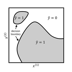
Figure 7.1. An example of a decision boundary in a feature space. The gray regions correspond to feature values for which the decision function predicts employees are skilled in serverless architecture. The white regions correspond to features for which the decision function predicts employees are unskilled in serverless architecture. The black lines are the decision boundary. Accessible caption. A stylized plot with the first feature dimension  on the horizontal axis and the second feature dimension  on the vertical axis. The space is partitioned into a couple of blob-like gray regions labeled  and a white region labeled . The boundary between the regions is marked as the decision boundary. Classifier regions do not have to be all one connected component.

Three key characteristics of a dataset determine how well the inductive biases of a classifier match the dataset:

1.    overlap of data points from the two class labels near the decision boundary,

2.    linearity or nonlinearity of the decision boundary, and

3.    number of data points, their density, and amount of clustering.

Classifier domains of competence are defined in terms of these three considerations.[4] Importantly, domains of competence are relative notions: does one classification algorithm work better than others?[5] They are not absolute notions, because at the end of the day, the absolute performance is limited by the Bayes optimal risk defined in Chapter 6. For example, one classification method that you tried may work better than others on datasets with a lot of class overlap near the decision boundary, nearly linear shape of the decision boundary, and not many data points. Another classification method may work better than others on datasets without much class overlap near a tortuously-shaped decision boundary. Yet another classification method may work better than others on very large datasets. In the remainder of this chapter, you will analyze many different supervised learning algorithms. The aim is not only describing how they work, but analyzing their inductive biases and domains of competence.

 

7.2           Two Ways to Approach Supervised Learning

Let’s begin by cataloging what you and the team of JCN Corporation data scientists have at your disposal. Your training dataset consists of  samples  independently drawn from the probability distribution . The features  sampled from the random variable  are numerical or categorical quantities derived from skill self-assessments, work artifacts, and so on. There are  features, so  is a -dimensional vector. The labels , sampled from the random variable  are the binary (zero or one) expertise evaluations on serverless architecture. Importantly, you do not have access to the precise distribution , but only to the finite number of samples contained in the training dataset drawn from the distribution. This is the key difference between the supervised machine learning problem and the Bayesian detection problem introduced in Chapter 6. The goal is the same in both the machine learning and detection problems: find a decision function  that predicts labels from features.

What are your options to find the classifier  based on the training data? You cannot simply minimize the Bayes risk functional or the probability of error directly, because that would rely on full knowledge of the probability distribution of the features and labels, which you do not have. You and the team have two options:

1.    plug-in approach: estimate the likelihood functions and prior probabilities from the training data, and plug them into the Bayes optimal likelihood ratio test described in Chapter 6, or

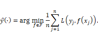
2.    risk minimization: optimize a classifier over an empirical approximation to the error rate computed on the training data samples.

There are specific methods within these two broad categories of supervised classification algorithms. A mental model for different ways of doing supervised machine learning is shown in Figure 7.2.

 

7.3           Plug-In Approach

First, you and the rest of the JCN Corporation data science team try out plug-in methods for supervised classification. The main idea is to use the training data to estimate the likelihood functions  and , and then plug them into the likelihood ratio to obtain the classifier.

7.3.1        Discriminant Analysis

One of the most straightforward plug-in methods, discriminant analysis, assumes a parametric form for the likelihood functions and estimates their parameters. Then just like in Chapter 6, it obtains a decision function by taking the ratio of these likelihood functions and comparing them to a threshold . The actual underlying likelihood functions do not have to be exactly their assumed forms and usually aren’t in practice. If they are somewhat close, that is good enough. The assumed parametric form is precisely the inductive bias of discriminant analysis.

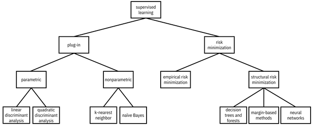
Figure 7.2. A mental model for different ways of approaching supervised machine learning. A hierarchy diagram with supervised learning at its root. Supervised learning has children plug-in and risk minimization. Plug-in has children parametric and nonparametric. Parametric has children linear discriminant analysis and quadratic discriminant analysis. Nonparametric has children k-nearest neighbor and naïve Bayes. Risk minimization has children empirical risk minimization and structural risk minimization. Structural risk minimization has children decision trees and forests, margin-based methods, and neural networks.

If the assumed parametric form for the likelihood functions is multivariate Gaussian in  dimensions with mean parameters  and  and covariance matrix parameters  and ,[6] then the first step is to compute their empirical estimates , , , and  from the training data, which you know how to do from Chapter 3. The second step is to plug those estimates into the likelihood ratio to get the classifier decision function. Under the Gaussian assumption, the method is known as quadratic discriminant analysis because after rearranging and simplifying the likelihood ratio, the quantity compared to a threshold turns out to be a quadratic function of . If you further assume that the two covariance matrices  and  are the same matrix , then the quantity compared to a threshold is even simpler: it is a linear function of , and the method is known as linear discriminant analysis.

Figure 7.3 shows examples of linear and quadratic discriminant analysis classifiers in  dimensions trained on the data points shown in the figure. The red diamonds are the employees in the training set unskilled at serverless architecture. The green squares are the employees in the training set skilled at serverless architecture. The domain of competence for linear and quadratic discriminant analysis is datasets whose decision boundary is mostly linear, with a dense set of data points of both class labels near that boundary.

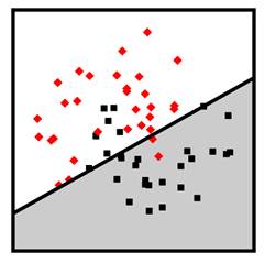
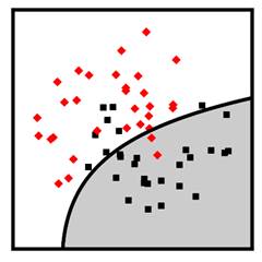
Figure 7.3. Examples of linear discriminant analysis (left) and quadratic discriminant analysis (right) classifiers. Accessible Caption. Stylized plot showing two classes of data points arranged in a noisy yin yang or interleaving moons configuration. The linear discriminant decision boundary is a straight line that cuts through the middle of the two classes. The quadratic discriminant decision boundary is a smooth curve that turns a little to enclose one of the classes.

7.3.2        Nonparametric Density Estimation

You continue your quest to analyze different classifiers for estimating the expertise of JCN employees. Instead of assuming a parametric form for the likelihood functions like in discriminant analysis, you try to estimate the likelihood functions in a nonparametric fashion. The word nonparametric is a misnomer. It does not mean that there are no parameters in the estimated likelihood function at all; it means that the number of parameters is on par with the number of training data points.

A common way of estimating a likelihood function nonparametrically is kernel density estimation. The idea is to place a smooth function like a Gaussian pdf centered on each of the training data points and take the normalized sum of those functions as the estimate of the likelihood function. In this case, the parameters are the centers of the smooth functions, so the number of parameters equals the number of data points. Doing this for both likelihood functions separately, taking their ratio, and comparing to a threshold yields a valid classifier. However, it is a pretty complicated classifier. You would need a lot of data to get a good kernel density estimate, especially when the data has a lot of feature dimensions .

Instead of doing the full density estimate, a simplification is to assume that all the feature dimensions of  are mutually independent. Under this assumption, the likelihood functions factor into products of one-dimensional pdfs that can be estimated separately with much less data. If you take the ratio of these products of one-dimensional pdfs (a likelihood ratio) and compare to a threshold, voilà, you have a naïve Bayes classifier. The name of this method contains ‘naïve’ because it is somewhat naïve to assume that all feature dimensions are independent—they never are in real life. It contains ‘Bayes’ because of plugging in to the Bayes-optimal likelihood ratio test. Often, this classifier does not outperform other classifiers in terms of accuracy, so its domain of competence is often non-existent.

A different nonparametric method is the k-nearest neighbor classifier. The idea behind it is very simple. Look at the labels of the  closest training data points and predict whichever label is more common in those nearby points. A distance metric is needed to measure ‘close’ and ‘near.’ Typically, Euclidean distance (the normal straight-line distance) is used, but other distance metrics could be used instead. The k-nearest neighbor method works better than other classifiers when the decision boundary is very wiggly and broken up into lots of components, and when there is not much overlap in the classes. Figure 7.4 shows examples of naïve Bayes and k-nearest neighbor classifiers in two dimensions. The k-nearest neighbor classifier in the figure has .

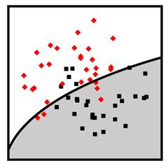
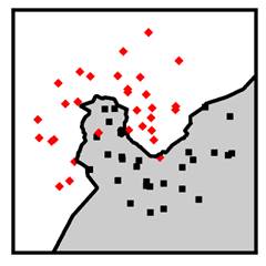
Figure 7.4. Examples of naïve Bayes (left) and k-nearest neighbor (right) classifiers. Accessible caption. Stylized plot showing two classes of data points arranged in a noisy yin yang or interleaving moons configuration. The naïve Bayes decision boundary is a smooth curve that turns a little to enclose one of the classes. The k-nearest neighbor decision boundary is very jagged and traces out the positions of the classes closely.

7.4           Risk Minimization Basics

You and the JCN team have tried out a few plug-in methods for your task of predicting which employees are skilled in serverless architecture and are ready to move on to a different category of machine learning methods: risk minimization. Whereas plug-in methods take one step back from the Bayes-optimal likelihood ratio test by estimating the likelihood functions from data, risk minimization takes two steps back and directly tries to find decision functions or decision boundaries that minimize an estimate of the Bayes risk.

7.4.1        Empirical Risk Minimization

Remember from Chapter 6 that the probability of error , the special case of the Bayes risk with equal costs that you’ve chosen as the performance metric, is:

Equation 7.1

The prior probabilities of the class labels  and  multiply the probabilities of the events when the decision function is wrong  and . You cannot directly compute the error probability because you do not have access to the full underlying probability distribution. But is there an approximation to the error probability that you can compute using the training data?

First, because the training data is sampled i.i.d. from the underlying distribution, the proportion of employees in the training data set skilled and unskilled at serverless architecture will approximately match the prior probabilities  and , so you do not have to worry about them explicitly. Second, the probabilities of both the false positive event  and false negative event  event can be expressed collectively as , which corresponds to  for training data samples. The zero-one loss function  captures this by returning the value  for  and the value  for . Putting all these things together, the empirical approximation to the error probability, known as the empirical risk , is:

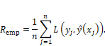
Equation 7.2

Minimizing the empirical risk over all possible decision functions  is a possible classification algorithm, but not one that you and the other JCN Corporation data scientists evaluate just yet. Let’s understand why not.

7.4.2        Structural Risk Minimization

Without any constraints, you can find a decision function that brings the empirical risk to zero but does not generalize well to new unseen data points. At the extreme, think about a classifier that memorizes the training data points and gets them perfectly correct, but always predicts  (unskilled at serverless architecture) everywhere else. This is not the desired behavior—the classifier has overfit. So just minimizing the empirical risk does not yield a competent classifier. This memorizing classifier is pretty complex. There’s nothing smooth or simple about it because it has as many discontinuities as there are training set employees skilled at serverless architecture.

Constraining the complexity of the classifier forces it to not overfit. To be a bit more precise, if you constrain the decision function  to be an element of some class of functions or hypothesis space  that only includes low-complexity functions, then you will prevent overfitting. But you can go too far with the constraints as well. If the hypothesis space is too small and does not contain any functions with the capacity to capture the important patterns in the data, it may underfit the data and not generalize either. It is important to control the hypothesis space to be just right. This idea is known as the structural risk minimization principle.

Figure 7.5 shows the idea in pictorial form using a sequence of nested hypothesis spaces . As an example of nested hypothesis spaces,  could be all constant functions,  could be all linear functions,  could be all quadratic functions, and  could be all polynomial functions.  contains the least complex  functions while  also contains more complex  functions.  underfits as it has large values for both the empirical risk  calculated on the training data and the probability of error , which measures generalization.  overfits as it has zero  and a large value for .  achieves a good balance and is just right.

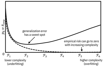
Figure 7.5. Illustration of the structural risk minimization principle. Accessible caption. A plot with  or  on the vertical axis and increasing complexity of hypothesis spaces on the horizontal axis. The empirical risk decreases all the way to zero with increasing complexity. The generalization error first decreases and then increases. It has a sweet spot in the middle.

The hypothesis space  is the inductive bias of the classifier. Thus, within the paradigm of the structural risk minimization principle, different choices of hypothesis spaces yield different domains of competence. In the next section, you and your team of JCN data scientists analyze several different risk minimization classifiers popularly used in practice, including decision trees and forests, margin-based classifiers (logistic regression, support vector machines, etc.), and neural networks.

 

7.5           Risk Minimization Algorithms

You are now analyzing the competence of some of the most popular classifiers used today that fit into the risk minimization paradigm. The basic problem is to find the function  within the hypothesis space  that minimizes the average loss function :

Equation 7.3

This equation may look familiar because it is similar to the Bayesian detection problem in Chapter 6. The function in the hypothesis space that minimizes the sum of the losses on the training data is . Different methods have different hypothesis spaces  and different loss functions . An alternative way to control the complexity of the classifier is not through changing the hypothesis space , but through a complexity penalty or regularization term  weighted by a regularization parameter :

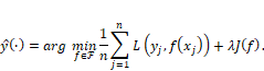
Equation 7.4

The choice of regularization term  also yields an inductive bias for you to analyze.

7.5.1        Decision Trees and Forests

One of the simplest hypothesis spaces is the set of decision stumps or one-rules. These classifiers create a single split along a single feature dimension like a numerical expertise self-assessment feature or a length of service feature. Any data point whose value is on one side of a threshold gets classified as skilled in serverless architecture, and on the other side as unskilled in serverless architecture. For categorical features, a split is just a partitioning of the values into two groups. The other features besides the one participating in the decision stump can be anything. An example of a decision stump is shown in Figure 7.6 as a node with two branches and also through its decision boundary.

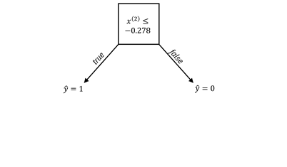
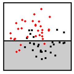
Figure 7.6. An example of a decision stump classifier. Accessible caption. On the left is a decision node . When it is true,  and when it is false, . On the right is a stylized plot showing two classes of data points arranged in a noisy yin yang or interleaving moons configuration. The decision boundary is a horizontal line. 

The hypothesis space of decision trees includes decision functions with more complexity than decision stumps. A decision tree is created by splitting on single feature dimensions within each branch of the decision stump, splitting within those splits, and so on. An example of a decision tree with two levels is shown in Figure 7.7. Decision trees can go much deeper than two levels to create fairly complex decision boundaries. An example of a complex decision boundary from a decision tree classifier is shown in Figure 7.8.

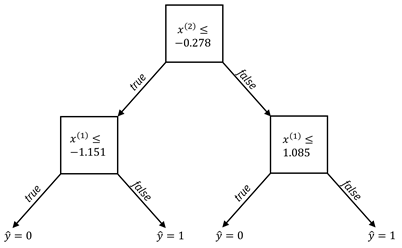
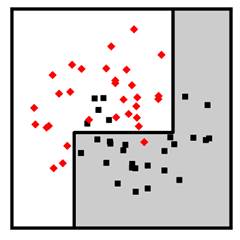
Figure 7.7. An example of a two-level decision tree classifier. Accessible caption. On the left is a decision node . When it is true, there is another decision node . When this decision node is true,  and when it is false, When the top decision node is false, there is another decision node . When this decision node is true,  and when it is false,  On the right is a stylized plot showing two classes of data points arranged in a noisy yin yang or interleaving moons configuration. The decision boundary is a made up of three line segments: the first segment is vertical, it turns right into a horizontal segment, and then up into another vertical segment.

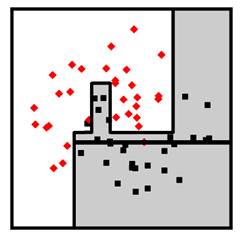
Figure 7.8. An example decision tree classifier with many levels. Accessible caption. A stylized plot showing two classes of data points arranged in a noisy yin yang or interleaving moons configuration. The decision boundary is a made up of several vertical and horizontal segments.

The hypothesis space of decision forests is made up of ensembles of decision trees that vote for their prediction, possibly with an unequal weighting given to different trees. The weighted majority vote from the decision trees is the overall classification. The mental model for a decision forest is illustrated in Figure 7.9 and an example decision boundary is given in Figure 7.10.

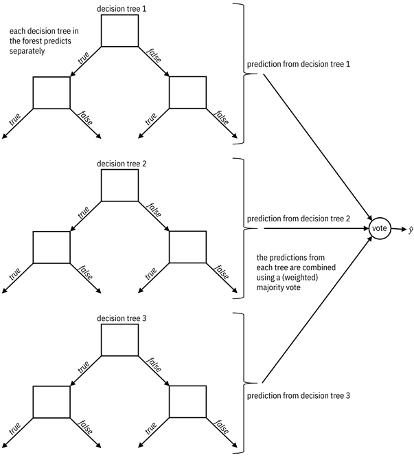
Figure 7.9. A mental model for a decision forest. Accessible caption. Three individual decision trees each predict separately. Their predictions feed into a vote node which outputs . The predictions from each tree are combined using a (weighted) majority vote.

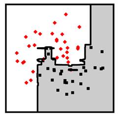
Figure 7.10. An example decision forest classifier. Accessible caption. Stylized plot showing two classes of data points arranged in a noisy yin yang or interleaving moons configuration. The decision boundary is fairly jagged with mostly axis-aligned segments and traces out the positions of the classes closely.

Decision stumps and decision trees can be directly optimized for the zero-one loss function that appears in the empirical risk.[7] More commonly, however, greedy heuristic methods are employed for learning decision trees in which the split for each node is done one at a time, starting from the root and progressing to the leaves. The split is chosen so that each branch is as pure as can be for the two classes: mostly just employees skilled at serverless architecture on one side of the split, and mostly just employees unskilled at serverless architecture on the other side of the split. The purity can be quantified by two different information-theoretic measures, information gain and Gini index, which were introduced in Chapter 3. Two decision tree algorithms are popularly-used: the C5.0 decision tree that uses information gain as its splitting criterion, and the classification and regression tree (CART) that uses Gini index as its splitting criterion. The depth of decision trees is controlled to prevent overfitting. The domain of competence of C5.0 and CART decision trees is tabular datasets in which the phenomena represented in the features tend to have threshold and clustering behaviors without much class overlap.

Decision forests are made up of a lot of decision trees. C5.0 or CART trees are usually used as these base classifiers. There are two popular ways to train decision forests: bagging and boosting. In bagging, different subsets of the training data are presented to different trees and each tree is trained separately. All trees have equal weight in the majority vote. In boosting, a sequential procedure is followed. The first tree is trained in the standard manner. The second tree is trained to focus on the training samples that the first tree got wrong. The third tree focuses on the errors of the first two trees, and so on. Earlier trees receive greater weight. Decision forests have good competence because of the diversity of their base classifiers. As long as the individual trees are somewhat competent, any unique mistake that any one tree makes is washed out by the others for an overall improvement in generalization.

The random forest classifier is the most popular bagged decision forest and the XGBoost classifier is the most popular boosted decision forest. Both have very large domains of competence. They are robust and work extremely well for almost all kinds of structured datasets. They are the first-choice algorithms for practicing data scientists to achieve good accuracy models with little to no tuning of parameters.

7.5.2        Margin-Based Methods

Margin-based classifiers constitute another popular family of supervised learning algorithms. This family includes logistic regression and support vector machines (SVMs). The hypothesis space of margin-based classifiers is more complex than decision stumps, but in a different way than decision trees. Margin-based classifiers allow any linear decision boundary rather than only ones parallel to single feature dimensions. Going even further, margin-based classifiers can have nonlinear decision boundaries in the original feature space by applying nonlinear functions to the features and finding linear decision boundaries in that transformed space.[8]

The main concept of these algorithms is the margin, the distance of data points to the decision boundary. With a linear decision boundary, the form of the classifier is [9] where  is a weight vector or coefficient vector that is learned from the training data. The absolute value of  is the distance of the data point to the decision boundary and is thus the margin of the point. The quantity  is positive if  is on one side of the hyperplane defined by  and negative if  is on the other side. The  function gives a classification of  (unskilled at serverless architecture) for negative margin and a classification of  (skilled at serverless architecture) for positive margin. The stuff with the  function (adding one and dividing by two) is just a way to recreate the behavior of the  function.

Surrogates for the zero-one loss function  are used in the risk minimization problem. Instead of taking two arguments, these margin-based loss functions take the single argument . When  is multiplied by , the result is positive for a correct classification and negative for an incorrect classification.[10] The loss is large for negative inputs and small or zero for positive inputs. In logistic regression, the loss function is the logistic loss:  and in SVMs, the loss function is the hinge loss: . The shape of these loss function curves is shown in Figure 7.11.

The regularization term  for the standard forms of logistic regression and SVMs is , the length-squared of the coefficient vector (also known as the -norm squared). The loss function, regularization term, and nonlinear feature mapping together constitute the inductive bias of the classifier. An alternative regularization term is the sum of the absolute values of the coefficients in (also known as the -norm), which provides the inductive bias for  to have many zero-valued coefficients. Example linear and nonlinear logistic regression and SVM classifiers are shown in Figure 7.12. The domain of competence for margin-based classifiers is fairly broad: structured datasets of moderate size. SVMs work a little better than logistic regression when the features are noisy.

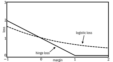
Figure 7.11. Margin-based loss functions. Accessible caption. A plot with loss on the vertical axis and margin on the horizontal axis. The logistic loss decreases smoothly. The hinge loss decreases linearly until the point , after which it is  for all larger values of the margin.

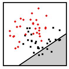
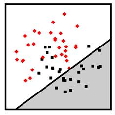
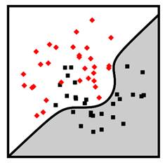
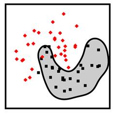
Figure 7.12. Example linear logistic regression (top left), linear SVM (top right), nonlinear polynomial SVM (bottom left), and nonlinear radial basis function SVM (bottom right) classifiers. Accessible caption. Stylized plot showing two classes of data points arranged in a noisy yin yang or interleaving moons configuration. The linear logistic regression and linear SVM decision boundaries are diagonal lines through the middle of the moons. The polynomial SVM decision boundary is a diagonal line with a smooth bump to better follow the classes. The radial basis function SVM decision boundary smoothly encircles one of the classes with a blob-like region.

7.5.3        Neural Networks

The final family of classifiers that you and the other JCN Corporation data scientists analyze is artificial neural networks. Neural networks are all the rage these days because of their superlative performance on high-profile tasks involving large-scale semi-structured datasets (image classification, speech recognition, natural language processing, bioinformatics, etc.), which is their domain of competence. The hypothesis space of neural networks includes functions that are compositions of compositions of compositions of simple functions known as neurons. The best way to understand the hypothesis space is graphically as layers of neurons, represented as nodes, connected to each other by weighted edges. There are three types of layers: an input layer, possibly several hidden layers, and an output layer. The basic picture to keep in mind is shown in Figure 7.13. The term deep learning which is bandied about quite a bit these days refers to deep neural networks: architectures of neurons with many many hidden layers.

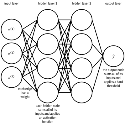
Figure 7.13. Diagram of a neural network. Accessible caption. Three nodes on the left form the input layer. They are labeled , , and   To the right of the input layer is hidden layer 1 with four nodes. To the right of hidden layer 1 is hidden layer 2 with four hidden nodes. To the right of hidden layer 2 is one node labeled  constituting the output layer. There are edges between each node of one layer and each node of the adjacent layer. Each edge has a weight. Each hidden node sums all of its inputs and applies an activation function. The output node sums all of its inputs and applies a hard threshold.

Logistic regression is actually a very simple neural network with just an input layer and an output node, so let’s start there. The input layer is simply a set of nodes, one for each of the  feature dimensions  relevant for predicting the expertise of employees. They have weighted edges coming out of them, going into the output node. The weights on the edges are the coefficients in , i.e. . The output node sums the weighted inputs, so computes , and then passes the sum through the  function. This overall procedure is exactly the same as logistic regression described earlier, but described in a graphical way.

In the regular case of a neural network with one or more hidden layers, nodes in the hidden layers also start with a weighted summation. However, instead of following the summation with an abrupt  function, hidden layer nodes use softer, more gently changing activation functions. A few different activation functions are used in practice, whose choice contributes to the inductive bias. Two examples, the sigmoid or logistic activation function  and the rectified linear unit (ReLU) activation function , are shown in Figure 7.14. The ReLU activation is typically used in all hidden layers of deep neural networks because it has favorable properties for optimization techniques that involve the gradient of the activation function.

 

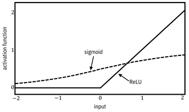
Figure 7.14. Activation functions. Accessible caption. A plot with activation function on the vertical axis and input on the horizontal axis. The sigmoid function is a gently rolling S-shaped curve that equals  at input value , approaches  as the input goes to negative infinity, and approaches  as the input goes to positive infinity. The ReLU function is  for all negative inputs and increases linearly starting at .

When there are several hidden layers, the outputs of nodes in one hidden layer feed into the nodes of the next hidden layer. Thus, the neural network’s computation is a sequence of compositions of weighted sum, activation function, weighted sum, activation function, and so on until reaching the output layer, which finally applies the  function. The number of nodes per hidden layer and the number of hidden layers is a design choice for JCN Corporation’s data scientists to make.

You and your team have analyzed the hypothesis space. Cool beans. The next thing for you to analyze is the loss function of neural networks. Recall that margin-based loss functions multiply the true label  by the distance  (not by the predicted label ), before applying the  function. The cross-entropy loss, the most common loss function used in neural networks, does kind of the same thing. It compares the true label  to a soft prediction  in the range  computed in the output node before the  function has been applied to it. The cross-entropy loss function is:

Equation 7.5

The form of the expression comes from cross-entropy, the average information in the true label random variable  when described using the predicted distance random variable , introduced in Chapter 3. Cross-entropy should be minimized because you want the description in terms of the prediction to be matched to the ground truth. It turns out that the cross-entropy loss is equivalent to the margin-based logistic loss function in binary classification problems, but it is pretty involved to show it mathematically because the margin-based loss function is a function of one variable that multiplies the prediction and the true label, whereas the two arguments are kept separate in cross-entropy loss.[11]

The last question to ask is about regularization. Although -norm, -norm, or other penalties can be added to the cross-entropy loss, the most common way to regularize neural networks is dropout. The idea is to randomly remove some nodes from the network on each iteration of an optimization procedure during training. Dropout’s goal is somewhat similar to bagging, but instead of creating an ensemble of several neural networks explicitly, dropout makes each iteration appear like a different neural network of an ensemble, which helps diversity and generalization. An example neural network classifier with one hidden layer and ReLU activation functions is shown in Figure 7.15. Repeating the statement from the beginning of this section, the domain of competence for artificial neural networks is semi-structured datasets with a large number of data points.

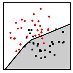
Figure 7.15. Example neural network classifier. Accessible caption. Stylized plot showing two classes of data points arranged in a noisy yin yang or interleaving moons configuration. The decision boundary is mostly smooth and composed of two almost straight diagonal segments that form a slightly bent elbow in the middle of the two moons.

7.5.4        Conclusion

You have worked your way through several different kinds of classifiers to compare and contrast their domains of competence and evaluate their appropriateness for your expertise assessment prediction task. Your dataset consists of mostly structured data, is of moderate size, and has a lot of feature axis-aligned separations between employees skilled and unskilled at serverless architecture. For these reasons, you can expect that XGBoost will be a competent classifier for your problem. But you should nevertheless do some amount of empirical testing of a few different methods.

 

7.6           Summary

§  There are many different methods for finding decision functions from a finite number of training samples, each with their own inductive biases for how they generalize.

§  Different classifiers have different domains of competence: what kinds of datasets they have lower generalization error on than other methods.

§  Parametric and non-parametric plug-in methods (discriminant analysis, naïve Bayes, k-nearest neighbor) and risk minimization methods (decision trees and forests, margin-based methods, neural networks) all have a role to play in practical machine learning problems.

§  It is important to analyze their inductive biases and domains of competence not only to select the most appropriate method for a given problem, but also to be prepared to extend them for fairness, robustness, explainability, and other elements of trustworthiness.