11
Adversarial Robustness
Imagine that you are a data scientist at a (fictional) new player in the human resources (HR) analytics space named HireRing. The company creates machine learning models that analyze resumes and metadata in job application forms to prioritize candidates for hiring and other employment decisions. They go in and train their algorithms on each of their corporate clients’ historical data. As a major value proposition, the executives of HireRing have paid extra attention to ensuring robustness to distribution shift and ensuring fairness of their machine learning pipelines and are now starting to focus their problem specification efforts on securing models from malicious acts. You have been entrusted to lead the charge in this new area of machine learning security. Where should you begin? What are the different threats you need to be worried about? What can you do to defend against potential adversarial attacks?
Adversaries are people trying to achieve their own goals to the detriment of the goals of HireRing and their clients, usually in a secretive way. For example, they may simply want to make the accuracy of an applicant prioritization model worse. They may be more sophisticated and want to trick the machine learning system into putting some small group of applicants at the top of the priority list irrespective of the employability expressed in their features while leaving the model’s behavior unchanged for most applicants.
This chapter teaches you all about defending and certifying the models HireRing builds for its clients by:
§ distinguishing different threat models based on what the adversary attacks (training data or models), their goals, and what they are privy to know and change,
§ defending against different types of attacks through algorithms that add robustness to models, and
§ certifying such robustness of machine learning pipelines.
The topic of adversarial robustness relates to the other two chapters in this part of the book on reliability (distribution shift and fairness) because it also involves a mismatch between the training data and the deployment data. You do not know what that difference is going to be, so you have epistemic uncertainty that you want to adapt to or be robust against. In distribution shift, the difference in distributions is naturally occurring; in fairness, the difference between a just world and the world we live in is because of encompassing societal reasons; in adversarial robustness, the difference between distributions is because of a sneaky adversary. Another viewpoint on adversarial attacks is not through the lens of malicious actors, but from the lens of probing system reliability—pushing machine learning systems to their extremes—by testing them in worst case scenarios. This alternative viewpoint is not the framing of the chapter, but you should keep it in the back of your mind and we will return to it in Chapter 13.
“In my view, similar to car model development and manufacturing, a comprehensive ‘in-house collision test’ for different adversarial threats on an AI model should be the new norm to practice to better understand and mitigate potential security risks.”
—Pin-Yu Chen, computer scientist at IBM Research
HireRing has just been selected by a large (fictional) retail chain based in the midwestern United States named Kermis to build them a resume and job application screening model. This is your first chance to work with a real client on the problem specification phase for adversarial robustness and not take any shortcuts. To start, you need to work through the different types of malicious attacks and decide how you can make the HireRing model being developed for Kermis the most reliable and trustworthy it can be. Later you’ll work on the modeling phase too.
11.1 The Different Kinds of Adversarial Attacks
As part of the problem specification phase for the machine learning-based job applicant classifier that HireRing is building for Kermis, you have to go in and assess the different threats it is vulnerable to. There are three dimensions by which to categorize adversarial attacks.[1] (1) Which part of the pipeline is being attacked: training or deployment? Attacks on training are known as poisoning attacks, whereas attacks on deployment are known as evasion attacks. (2) What capabilities does the attacker have? What information about the data and model do they know? What data and models can they change and in what way? (3) What is the goal of the adversary? Do they simply want to degrade performance of the resume screening model in general or do they have more sophisticated and targeted objectives? These three dimensions are similar to the three considerations when picking a bias mitigation algorithm in Chapter 10 (part of pipeline, presence of protected attributes, worldview).
A mental model of the different attack types is shown in Figure 11.1. Let’s go through each of the dimensions in turn as a sort of checklist to analyze what Kermis should most be worried about and what the HireRing model should protect against most diligently.
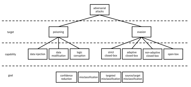
Figure 11.1. A mental model for the different types of adversarial attacks, according to their target, their capability, and their goal. A hierarchy diagram with adversarial attacks at its root. Adversarial attacks has children poisoning and evasion, both of which are in the target dimension. Poisoning has children data injection, data modification, and logic corruption, which are in the capability dimension. Evasion has children strict closed-box, adaptive closed-box, non-adaptive closed-box, and open-box, which are in the capability dimension. Below the hierarchy diagram are items in the goal dimension: confidence reduction, misclassification, targeted misclassification, and source/target misclassification, which apply to the whole diagram.
11.1.1 Target
Adversaries may target either the modeling phase or the deployment phase of the machine learning lifecycle. By attacking the modeling phase, they can corrupt the training data or model so that it is mismatched from the data seen in deployment. These are known as poisoning attacks and have similarities with distribution shift, covered in Chapter 9, as they change the statistics of the training data or model. Evasion attacks that target the deployment phase are a different beast that do not have a direct parallel with distribution shift, but have a loose similarity with individual fairness covered in Chapter 10. These attacks are focused on altering individual examples (individual resumes) that are fed into the machine learning system to be evaluated. As such, modifications to single data points may not affect the deployment probability distribution much at all, but can nevertheless achieve the adversary’s goals for a given input resume.
One
way to understand poisoning and evasion attacks is by way of the decision
boundary, shown in Figure 11.2. Poisoning attacks shift the decision boundary
in a way that the adversary wants. In contrast, evasion attacks do not shift
the decision boundary, but shift data points across the decision boundary in
ways that are difficult to detect. An original data point, the features of the
resume ![]() , shifted by
, shifted by ![]() becomes
becomes ![]() . A basic
mathematical description of an evasion attack is the following:
. A basic
mathematical description of an evasion attack is the following:
![]()
Equation 11.1
The
adversary wants to find a small perturbation ![]() to add to the resume
to add to the resume
![]() so that the
predicted label changes (
so that the
predicted label changes (![]() ) from select to
reject or vice versa. In addition, the perturbation should be smaller in length
or norm
) from select to
reject or vice versa. In addition, the perturbation should be smaller in length
or norm ![]() than some small
value
than some small
value ![]() . The choice of
norm and value depend on the application domain. For semi-structured data
modalities, the norm should capture human perception so that the perturbed data
point and the original data point look or sound almost the same to people.
. The choice of
norm and value depend on the application domain. For semi-structured data
modalities, the norm should capture human perception so that the perturbed data
point and the original data point look or sound almost the same to people.
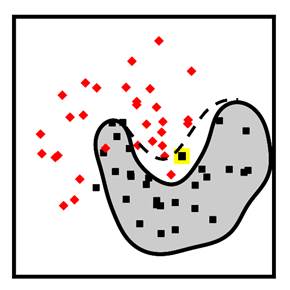
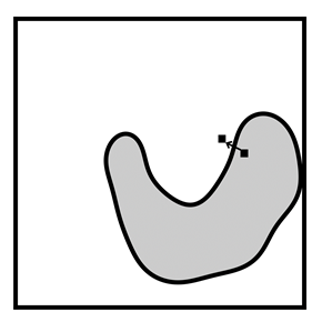
Figure 11.2. Examples of a poisoning attack (left) and an evasion attack (right). In the poisoning attack, the adversary has injected a new data point, the square with the light border into the training data. This action shifts the decision boundary from what it would have been: the solid black line, to something else that the adversary desires: the dashed black line. More diamond deployment data points will now be misclassified. In the evasion attack, the adversary subtly perturbs a deployment data point across the decision boundary so that it is now misclassified. Accessible caption. The stylized plot illustrating a poisoning attack shows two classes of data points arranged in a noisy yin yang or interleaving moons configuration and a decision boundary smoothly encircling one of the classes with a blob-like region. A poisoning data point with the label of the inside of the region is added outside the region. It causes a new decision boundary that puts it inside, while also causing the misclassification of another data point. The stylized plot illustrating the evasion attack has a data point inside the blob-like region. The attack pushes it outside the region.
Another
way to write the label change ![]() is through the
zero-one loss function:
is through the
zero-one loss function: ![]() . (Remember that
the zero-one loss takes value
. (Remember that
the zero-one loss takes value ![]() when both
arguments are the same and value
when both
arguments are the same and value ![]() when the arguments
are different.) Because the zero-one loss can only take the two values
when the arguments
are different.) Because the zero-one loss can only take the two values ![]() and
and ![]() , you can also write the adversarial
example using a maximum as:
, you can also write the adversarial
example using a maximum as:
![]()
Equation 11.2
In this notation, you can also put in other loss functions such as cross-entropy loss, logistic loss, and hinge loss from Chapter 7.
11.1.2 Capability
Some adversaries are more capable than others. In the poisoning category, adversaries change the training data or model somehow, so they have to have some access inside Kermis’ information technology infrastructure. The easiest thing they can do is slip in some additional resumes that get added to the training data. This is known as data injection. More challenging is data modification, in which the adversary changes labels or features in the existing training dataset. The most challenging of all is logic corruption, in which the adversary changes the code and behavior of the machine learning algorithm or model. You can think of the data injection and data modification attacks as somewhat similar to bias mitigation pre-processing and logic corruption as somewhat similar to bias mitigation in-processing, except for a nefarious purpose.
In
the evasion category, the adversary does not need to change anything at all
inside Kermis’ systems. So these are easier attacks to carry out. The attackers
just have to create adversarial examples: specially crafted resumes designed in
clever ways to fool the machine learning system. But how adversaries craft
these tricky resumes depends on what information they have about how the model
makes its predictions. The easiest thing for an adversary to do is just submit a
bunch of resumes into the HireRing model and see whether they get selected or
not; this gives the adversary a labeled dataset. When adversaries cannot change
the set of resumes and just have to submit a batch that they have, it is called
strict closed-box access. When they can change the
input resumes based on the previous ones they’ve submitted and the predicted
labels they’ve observed, it is called adaptive closed-box
access. Adaptivity is a bit harder because the attacker might have to wait a
while for Kermis to select or not select the resumes that they’ve submitted.
You might also be able to catch on that something strange is happening over
time. The next more difficult kind of information that adversaries can have
about the HireRing model trained for Kermis is known as non-adaptive
closed-box access. Here, the adversary knows the training data distribution
![]() but cannot submit
resumes. Finally, the classifier decision function itself
but cannot submit
resumes. Finally, the classifier decision function itself ![]() is the most
difficult-to-obtain information about a model for an adversary. This full
knowledge of the classifier is known as open-box
access.
is the most
difficult-to-obtain information about a model for an adversary. This full
knowledge of the classifier is known as open-box
access.
Since Kermis has generally good cybersecurity overall, you should be less worried about poisoning attacks, especially logic corruption attacks. Even open-box access for an evasion attack seems less likely. Your biggest fear should be one of the closed-box evasion attacks. Nevertheless, you shouldn’t let your guard down and you should still think about defending against all of the threats.
11.1.3 Goal
The
third dimension of threats is the goal of the adversary, which applies to both
poisoning and evasion attacks. Different adversaries try to do different
things. The easiest goal is confidence reduction: to
shift classifier scores so that they are closer to the middle of the range ![]() and thus less
confident. The next goal is misclassification:
trying to get the classifier to make incorrect predictions. (This is the
formulation given in Equation 11.1.) Job applications to Kermis that should be
selected are rejected and vice versa. When you have a binary classification
problem like you do in applicant screening, there is only one way to be wrong:
predicting the other label. However, when you have more than two possible
labels, misclassification can produce any other label that is not the true one.
Targeted misclassification goes a step further and
ensures that the misclassification isn’t just any other label, but a specific
one of the attacker’s choice. Finally, and most sophisticated of all, source/target misclassification attacks are designed so
that misclassification only happens for some input job applications and the
label of the incorrect prediction also depends on the input. Backdoor or Trojan attacks are an
example of source/target misclassification in which a small subset of inputs
(maybe ones whose resumes include some special keyword) trigger the application
to be accepted. The more sophisticated goals are harder to pull off, but also
the most dangerous for Kermis and HireRing if successful. The problem
specification should include provisions to be vigilant for all these different
goals of attacks.
and thus less
confident. The next goal is misclassification:
trying to get the classifier to make incorrect predictions. (This is the
formulation given in Equation 11.1.) Job applications to Kermis that should be
selected are rejected and vice versa. When you have a binary classification
problem like you do in applicant screening, there is only one way to be wrong:
predicting the other label. However, when you have more than two possible
labels, misclassification can produce any other label that is not the true one.
Targeted misclassification goes a step further and
ensures that the misclassification isn’t just any other label, but a specific
one of the attacker’s choice. Finally, and most sophisticated of all, source/target misclassification attacks are designed so
that misclassification only happens for some input job applications and the
label of the incorrect prediction also depends on the input. Backdoor or Trojan attacks are an
example of source/target misclassification in which a small subset of inputs
(maybe ones whose resumes include some special keyword) trigger the application
to be accepted. The more sophisticated goals are harder to pull off, but also
the most dangerous for Kermis and HireRing if successful. The problem
specification should include provisions to be vigilant for all these different
goals of attacks.
11.2 Defenses Against Poisoning Attacks
Once you and the HireRing team are in the modeling phase of the lifecycle, you have to implement defense measures against the attacks identified in the problem specification phase. From a machine learning perspective, there are no specific defenses for preventing logic corruption attacks in Kermis’ systems. They must be prevented by other security measures. There are, however, defenses throughout the machine learning pipeline against data injection and data modification attacks that fall into three categories based on where in the pipeline they are applied.[2] (1) Pre-processing approaches are given the name data sanitization. (2) In-processing defenses during model training rely on some kind of smoothing. (3) Post-processing defenses are called patching. These three categories, which are detailed in the remainder of this section, are illustrated in Figure 11.3. They are analogous to methods for mitigating distribution shift and unwanted bias described in Chapter 9 and Chapter 10, respectively.
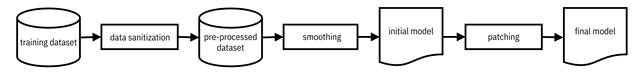
Figure 11.3. Different categories of defenses against poisoning attacks in the machine learning pipeline. Accessible caption. A block diagram with a training dataset as input to a data sanitization block with a pre-processed dataset as output. The pre-processed dataset is input to a smoothing block with an initial model as output. The initial model is input to a patching block with a final model as output.
Machine learning defenses against poisoning attacks are an active area of research. Specific attacks and defenses are continually improving in an arms race. Since by the time this book comes out, all presently known attacks and defenses are likely to have been superseded, only the main ideas are given rather than in-depth accounts.
11.2.1 Data Sanitization
The main idea of data sanitization is to locate the nefarious resumes that have been injected into or modified in the Kermis dataset and remove them. Such resumes tend to be anomalous in some fashion, so data sanitization reduces to a form of anomaly or outlier detection. The most common way to detect outliers, robust statistics, is as follows. The set of outliers is assumed to have small cardinality compared to the clean, unpoisoned training resumes. The two sets of resumes, poison and clean, are differentiated by having differing means normalized by their variances. Recent methods are able to differentiate the two sets efficiently even when the number of features is large.[3] For high-dimensional semi-structured data, the anomaly detection should be done in a representation space rather than in the original input feature space. Remember from Chapter 4 that learned representations and language models compactly represent images and text data, respectively, using the structure they contain. Anomalies are more apparent when the data is well-represented.
11.2.2 Smoothing
When HireRing is training the Kermis classifier, defenses against data poisoning make the model more robust by smoothing the score function. The general idea is illustrated in Figure 11.4, which compares a smooth and less smooth score function. By preferring smooth score functions during training, there is a lower chance for adversaries to succeed in their attacks.
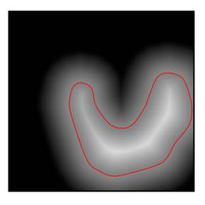
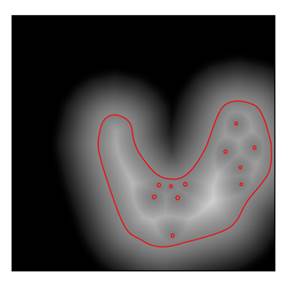
Figure 11.4. A comparison of a smooth (left) and less
smooth (right) score function. The value of the score function is indicated by
shading: it is ![]() where the shading
is white and
where the shading
is white and ![]() where the shading
is black. The decision boundary, where the score function takes value
where the shading
is black. The decision boundary, where the score function takes value ![]() is indicated by
red lines. The less smooth score function may have been attacked. Accessible
caption. Stylized plot showing a decision boundary smoothly encircling one of
the classes with a blob-like region. The underlying score function is indicated
by shading, becoming smoothly whiter in the inside the region and smoothly
blacker outside the region. This is contrasted with another decision boundary
that has some tiny enclaves of the opposite class inside the blob-like region.
Its underlying score function is not smooth.
is indicated by
red lines. The less smooth score function may have been attacked. Accessible
caption. Stylized plot showing a decision boundary smoothly encircling one of
the classes with a blob-like region. The underlying score function is indicated
by shading, becoming smoothly whiter in the inside the region and smoothly
blacker outside the region. This is contrasted with another decision boundary
that has some tiny enclaves of the opposite class inside the blob-like region.
Its underlying score function is not smooth.
Smoothing can be done, for example, by applying a k-nearest neighbor prediction on top of another underlying classifier. By doing so, the small number of poisoned resumes are never in the majority of a neighborhood and their effect is ignored. Any little shifts in the decision boundary stemming from the poisoned data points are removed. Another way to end up with a smooth score function, known as gradient shaping, is by directly constraining or regularizing its slope or gradient within the learning algorithm. When the magnitude of the gradient of a decision function is almost the same throughout the feature space, it is resilient to perturbations caused by a small number of anomalous points: it is more like the left score function in Figure 11.4 than the right score function. Smoothing can also be accomplished by averaging together the score functions of several independent classifiers.
11.2.3 Patching
Patching, primarily intended for neural network models, mitigates the effect of backdoor attacks as a post-processing step. Backdoors show up as anomalous edge weights and node activations in neural networks. There is something statistically weird about them. Say that you have already trained an initial model on a poisoned set of Kermis job applications that has yielded a backdoor. The idea of the patching is similar to how you fix a tear in a pair of pants. First you ‘cut’ the problem out of the ‘fabric’: you prune the anomalous neural network nodes. Then you ‘sew’ a patch over it: you fine-tune the model with some clean resumes or a set of resumes generated to approximate a clean distribution.
11.3 Defenses Against Evasion Attacks
Evasion
attacks are logistically simpler to carry out than poisoning attacks because
they do not require the adversary to infiltrate Kermis’ information technology
systems. Adversaries only have to create examples that look realistic to avoid
suspicion and submit them as regular job applications. Defending against these
attacks can be done in two main ways: (1) denoising and (2) adversarial
training. The first category of defenses is outside the machine learning
training pipeline and applies at deployment. It tries to subtract off the
perturbation ![]() from a deployment-time
resume
from a deployment-time
resume ![]() when it exists.
(Only a small number of input resumes will be adversarial examples and have a
when it exists.
(Only a small number of input resumes will be adversarial examples and have a ![]() .) This first
category is known as denoising; the reason will
become apparent in the next section. The second category of defenses occurs in
the modeling pipeline and builds min-max robustness into the model itself,
similar to training models robust to distribution shift in Chapter 9. It is
known as adversarial training. There is no evasion
defense category analogous to adaptation or bias mitigation pre-processing of
training data from Chapter 9 and Chapter 10, respectively, because evasion
attacks are not founded in training data distributions. The defenses to evasion
attacks are summarized in Figure 11.5. Let’s learn more about implementing
these defenses in the HireRing job applicant prioritization system.
.) This first
category is known as denoising; the reason will
become apparent in the next section. The second category of defenses occurs in
the modeling pipeline and builds min-max robustness into the model itself,
similar to training models robust to distribution shift in Chapter 9. It is
known as adversarial training. There is no evasion
defense category analogous to adaptation or bias mitigation pre-processing of
training data from Chapter 9 and Chapter 10, respectively, because evasion
attacks are not founded in training data distributions. The defenses to evasion
attacks are summarized in Figure 11.5. Let’s learn more about implementing
these defenses in the HireRing job applicant prioritization system.
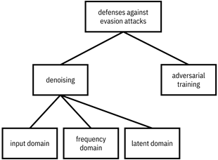
Figure 11.5. Different defenses against evasion attacks. Accessible caption. A hierarchy diagram with defenses against evasion attacks at its root, which has denoising and adversarial training as its children. Denoising has children input domain, frequency domain, and latent domain.
11.3.1 Denoising Input Data
Despite
the best efforts of attackers, adversarial examples—resumes that have been
shifted across a decision boundary—contain signals noticeable by machines even
though they are imperceptible for people. The specially-crafted perturbation ![]() is a form of
noise, called adversarial noise. Denoising,
attempting to remove
is a form of
noise, called adversarial noise. Denoising,
attempting to remove ![]() from
from
![]() ,
is a type of defense. The challenge in denoising is to remove
all of the noise while limiting the distortion to the underlying clean
features.
,
is a type of defense. The challenge in denoising is to remove
all of the noise while limiting the distortion to the underlying clean
features.
Noise removal is an old problem that has been addressed in signal processing and related fields for a long time. There are three main ways of denoising evasion attacks that differ in their representation of the data: (1) input domain, (2) frequency domain, and (3) latent domain.[4] Denoising techniques working directly in the feature space or input domain may copy or swap feature values among neighboring data points. They may also quantize continuous values into a smaller set of discrete values. Taking advantage of recent advances in generative machine learning (briefly described in Chapter 4 in the context of data augmentation), they may generate data samples very similar to an input, but without noise. Taken together, the main idea for input domain denoising is to flatten the variability or smooth out the data values.
Smoothing is better examined in the frequency domain. If you are not an electrical engineer, you might not have heard about converting data into its frequency domain representation. The basic idea is to transform the data so that very wiggly data yields large values at so-called high frequencies and very smooth data yields large values at the opposite end of the spectrum: low frequencies. This conversion is done using the Fourier transform and other similar operations. Imperceptible adversarial noise is usually concentrated at high frequencies. Therefore, a defense for evasion attacks is squashing the high frequency components of the data (replacing them with small values) and then converting the data back to the input domain. Certain data compression techniques for semi-structured data modalities indirectly accomplish the same thing.
If your machine learning model is a neural network, then the values of the data as it passes through intermediate layers constitute a latent representation. The third denoising category works in this latent representation space. Like in the frequency domain, this category also squashes the values in certain dimensions. However, these techniques do not simply assume that the adversarial noise is concentrated in a certain part of the space (e.g. high frequencies), but learn these dimensions using clean job applications and their corresponding adversarial examples that you create.
11.3.2 Adversarial Training
The second main category of defenses against evasion attacks is adversarial training. It is a form of min-max robustness,[5] which you first encountered in Chapter 9 in the context of distribution shift. Remember that the min-max idea is to do the best you can on the worst-case scenario. In adversarial training, the minimization and maximization are as follows. The minimization is to find the best job applicant classifier in the hypothesis space, just like any other risk minimization approach to machine learning. The inner maximization is to find the worst-case perturbations of the resumes. The mathematical form of the objective is:
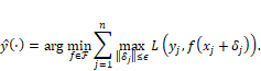
Equation 11.3
Notice that the inner maximization is the same expression as finding adversarial examples given in Equation 11.2. Thus, to carry out adversarial training, all you have to do is produce adversarial examples for the Kermis training resumes and use those adversarial examples as a new training data set in a typical machine learning algorithm. HireRing must become a good attacker to become a good defender.
11.3.3 Evaluating and Certifying Robustness to Evasion Attacks
Once the HireRing job applicant screening system has been adversarially trained on Kermis resumes, how do you know it is any good? There are two main ways to measure the model’s robustness: (1) empirically and (2) characterizing the score function. As an empirical test, you create your own adversarial example resumes, feed them in, and compute how often the adversarial goal is met (confidence reduction, misclassification, targeted misclassification, or source/target misclassification). You can do it because you know the ground truth of which input resumes contain an adversarial perturbation and which ones don’t. Such empirical robustness evaluation is tied to the specific attack and its capabilities (open-box or closed-box) since you as the evaluator are acting as the adversary.
In
contrast, a way to characterize the adversarial robustness of a classifier that
is agnostic to the evasion attack is the CLEVER score.[6]
An acronym for cross-Lipschitz extreme value for network robustness, the CLEVER
score (indirectly) analyzes the distance from a job application data point to
the classifier decision boundary. Misclassification attacks will be
unsuccessful if this distance is too far because it will exceed ![]() , the bound on the
norm of the perturbation
, the bound on the
norm of the perturbation ![]() . The higher the CLEVER
score, the more robust the model. Generally speaking, smooth, non-complicated decision
boundaries without many small islands (like the left score function in Figure
11.4) have large distances from data points on average, have large average
CLEVER scores, and are robust to all kinds of evasion attacks. In the problem
specification phase with the Kermis problem owners, you can set an acceptable
minimum value for the average CLEVER score. If the model achieves it, HireRing
can confidently certify a level of security and robustness.
. The higher the CLEVER
score, the more robust the model. Generally speaking, smooth, non-complicated decision
boundaries without many small islands (like the left score function in Figure
11.4) have large distances from data points on average, have large average
CLEVER scores, and are robust to all kinds of evasion attacks. In the problem
specification phase with the Kermis problem owners, you can set an acceptable
minimum value for the average CLEVER score. If the model achieves it, HireRing
can confidently certify a level of security and robustness.
11.4 Summary
§ Adversaries are actors with bad intentions who try to attack machine learning models by degrading their accuracy or fooling them.
§ Poisoning attacks are implemented during model training by corrupting either the training data or model.
§ Evasion attacks are implemented during model deployment by creating adversarial examples that appear genuine, but fool models into making misclassifications.
§ Adversaries may just want to worsen model accuracy in general or may have targeted goals that they want to achieve, such as obtaining specific predicted labels for specific inputs.
§ Adversaries have different capabilities of what they know and what they can change. These differences in capabilities and goals determine the threat.
§ Defenses for poisoning attacks take place at different parts of the machine learning pipeline: data sanitization (pre-processing), smoothing (model training), and patching (post-processing).
§ Defenses for evasion attacks include denoising that attempts to remove adversarial perturbations from inputs and adversarial training which induces min-max robustness.
§ Models can be certified for robustness to evasion attacks using the CLEVER score.
§ Even without malicious actors, adversarial attacks are a way for developers to test machine learning systems in worst case scenarios.